Documentation
Thin Film Forge designs, analyzes, fits and tolerances optical interference coatings: anti-reflection coatings, edge, band-pass and notch filters, and mirrors, from the UV to the long-wave infrared.
You are reading the public documentation. Production and advanced sections are shortened: sign up now (free) or sign in to read everything.
Quick start
- Open the app. The design library opens on first visit with 37 designs from the literature
(later: File › Open from library or L). File › New film starts from a substrate and an H/L stack instead.
When the library closes, a short tour points out the main parts of the window, one click each (Help › Tour of
the app runs it again).
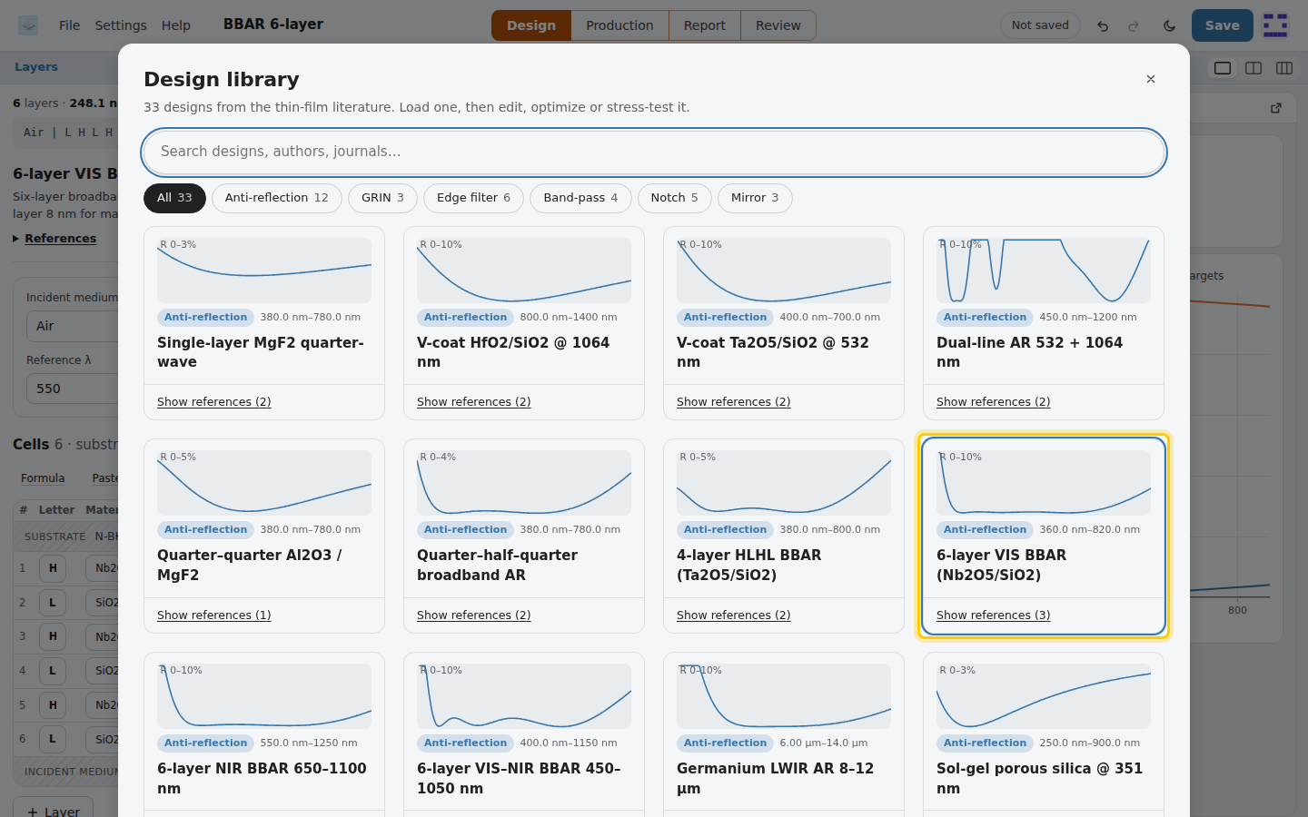
The design library. Pick a design to load it. - Pick one. The Layers panel on the left shows its layers, the center shows the spectrum, and the bar along the
bottom holds Requirements and Optimize.
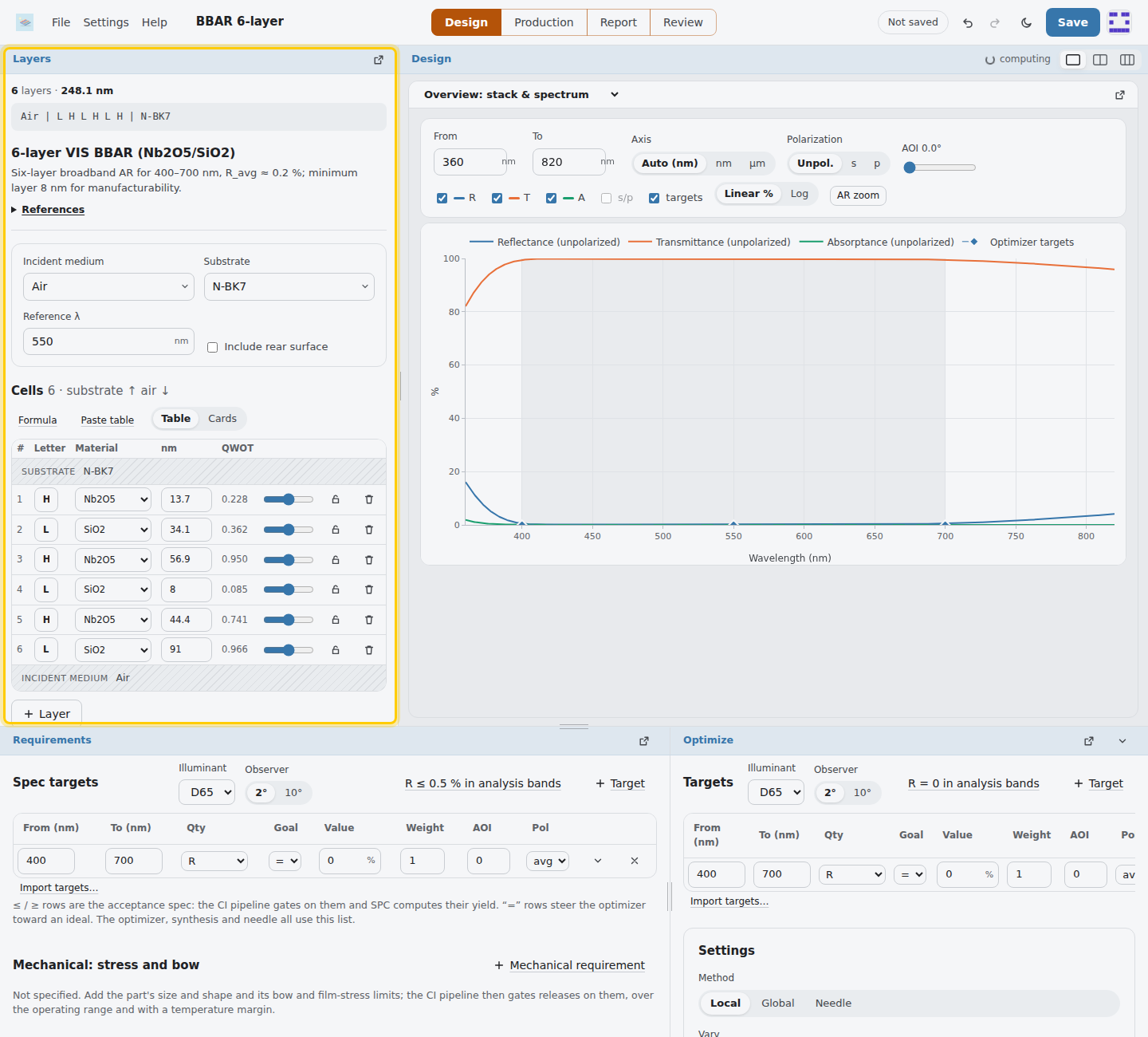
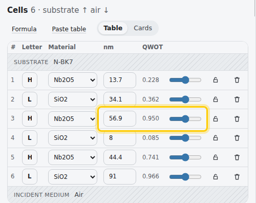
The Layers panel: medium, substrate, reference wavelength and the cells. - Drag a thickness slider or change a material: everything recalculates as you edit. GRIN designs recalculate
when you press Recalculate, and the thermal, stress and ultrafast views when you press it or turn on Auto. Ctrl+Z undoes.
Each cell has a thickness in nm or quarter-waves, and a slider. - The tabs along the top switch sections: Design (Layers in the side bar; Thermal and Stress & bow
in the panes), Production (Fit data, Characterize, Monitoring, Run sheet, SPC / yield), Report
(the EIDP report) and Review (read-only review and comparison of revisions, History & releases).
The center shows one or two panes (Alt+1 / 2), or a custom
grid of up to 3 × 3 picked from the starred box (Alt+3), each pane picking its
view from the menu in its header. The menu bar holds File, Settings (Advanced design and the Materials library under
Advanced) and Help; its menus work from the keyboard: arrow keys move between and within them,
Esc closes.

The section tabs along the top; the picker at the right sets one or two panes, or a custom grid.
Your work autosaves in the browser. File › Save (Ctrl+S) commits it to version control, Save as (Ctrl+Shift+S) starts a new tracked design under another name, and File › Export writes a design file, the layer table, the spectrum, the audit package or a share link.

Building a design
A design is a stack of cells on a substrate, listed from the substrate outward (the editor shows the air side on top). Choose the incident medium, the substrate and a reference wavelength; the reference is used for quarter-wave (QWOT) entry, the index profile and the admittance diagram.
Cells
| Kind | What it is |
|---|---|
| Layer | A homogeneous film. Enter physical thickness in nm or optical thickness in quarter-waves at the reference wavelength. |
| GRIN linear / cubic / quintic | A graded-index ramp between material A (\(f = 0\)) and B (\(f = 1\)), split into sub-layers. Quintic is Southwell's ripple-free profile. |
| GRIN rugate | A sinusoidal index profile set by its notch wavelength, cycles and amplitude, with Gaussian, quintic or half-sine apodization. |
GRIN cells mix their two materials by linear index or by Bruggeman effective-medium theory (porous or co-deposited films). A GRIN cell with the same composition at both ends is a homogeneous mixture layer.
Repeat blocks
Repeat any contiguous range of cells \(N\) times. Blocks may nest, so a two-cavity band-pass
[(HL)^4 HH (LH)^4 L]^2 needs only six cells. The formula line above the editor shows the result.
Long stacks
Designs can hold up to 400 cells. The editor lists them in a compact table; Cards shows one card per cell instead (also when the side bar is too narrow for the table). Paste table accepts a layer list copied from a paper or spreadsheet, one layer per line, substrate side first:
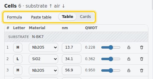
GaAs 340.0
Al0.92Ga0.08As 388.6
ta2o5, 112.4
L 183.0
Materials may be given by id, name, chemical formula, algaas:x, or H / L / M for Ta₂O₅ / SiO₂ / Al₂O₃.
Designs can hold up to 5,000 cells per side; the table shows them in pages.
Stack formulas
Formula builds a stack from notation, substrate side first. Each letter is one quarter-wave at \(\lambda_0\) of the material
it is mapped to (\(n d = \lambda_0/4\)), a number multiplies what follows, and ^N repeats:
0.5L (HL)^8 H              long-wave-pass core
(HL)^5 1.2(HL)^5            two staggered mirrors
((HL)^4 4H (LH)^4 L)^2      nested groups
Groups become repeat blocks; a 41-layer mirror is a few cells.
Rear surface and environment
Rear face says how the substrate's back is seen, as the sample was measured:
- OFF: single-side polished (SSP, rough back), wedged or index-matched. Only the front face counts.
- ON: double-side polished (DSP); the rear reflection adds in intensity, including the substrate's absorption. Use it for thick parts, or when the instrument's resolution is coarser than the fringes.
The rear can be uncoated, carry the same stack as the front, or any AR coating from the library. Environment & temperature sets the operating and design temperatures (see Temperature).
Materials
The library holds 153 dispersive materials: glasses and crystals from their Sellmeier fits, oxide and fluoride films, \(\mathrm{Al}_x\mathrm{Ga}_{1-x}\mathrm{As}\)
from the Afromowitz model (any composition via algaas:0.35), IR materials, and Lorentz–Drude metals. Most of them are
published data sets vendored from the refractiveindex.info database (CC0), each cited in the Source column:
- Process-specific films: e-beam MgF₂, HfO₂, TiO₂ and Al₂O₃ (Franta), IAD and sputtered SiO₂ (Gao, Lemarchand), sputtered Nb₂O₅, Sc₂O₃ and AlN, ALD TiO₂, LaF₃, SiO, Y₂O₃, cubic ZrO₂, ZnO and ZnSe films.
- Conductive films: ITO and TiN.
- Metals: Cr, Ni, Pt, Ti, Pd, W, Be (Rakić), Mo (Werner), Rh (Weaver), and Cu, Co, Fe, Ag and Au (Johnson & Christy).
- Substrates: BOROFLOAT 33, D 263 T, EAGLE XG, ZERODUR, N-SF6, F2 and N-LASF9; sapphire (e-ray), crystal quartz, YAG, LiNbO₃, BaF₂, MgF₂, LiF, NaCl, KBr, CsI, KRS-5, diamond and MgO; InP, GaP and CdTe; AMTIR-1, IRG 22 and As₂S₃.
Each material is valid over its data set's own wavelength range, shown in the Valid column. Indices are checked in the test suite against handbook values.
- Mid-infrared films. Oxide films switch beyond 2 µm to measured film data (Kischkat 2012, Bright 2013, Franta 2025), so their vibrational absorption bands, such as SiO₂ near 9.3 µm, are included.
- Thermal constants. Every material carries \(\mathrm{d}n/\mathrm{d}T\), expansion coefficient \(\alpha\) and Poisson ratio \(\nu\). Film values are process-dependent starting points.
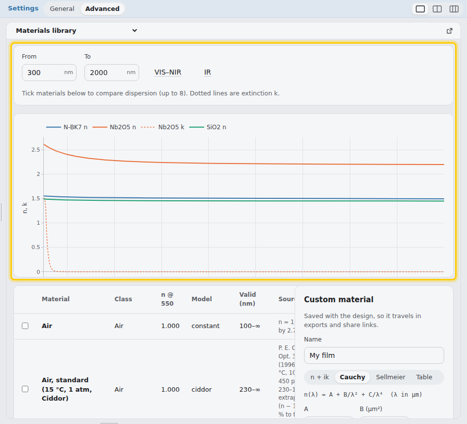
- Custom materials. Add constant \(n + ik\), Cauchy, Sellmeier or tabulated materials in Settings › Advanced › Materials library, with optional \(\mathrm{d}n/\mathrm{d}T\), expansion and Poisson ratio. Custom materials are saved with the design and frozen into every design record.
Measured n,k data
Choose Table under Custom material, then open a file or paste it and press Read data. The importers are:
| Format | Reads |
|---|---|
Columns (.csv .tsv .txt .dat .nk) | \(\lambda, n, k\) or \(\lambda, \varepsilon_1, \varepsilon_2\); with two columns \(k = 0\). The wavelength unit comes from the header (nm, µm, Å, eV, cm⁻¹) or the λ unit menu. Without either, values below 30 are read as µm. |
| refractiveindex.info YAML | Tabulated \(n\), \(k\) or \(nk\) blocks, or any of its dispersion formulas 1–9 (Sellmeier, Cauchy-type power series, gases, Herzberger, retro, exotic), sampled over its stated range. |
WVASE / CompleteEASE .mat | Title line, unit line (nm, eV, microns, 1/cm, Å), NK or E1E2, then rows. |
No extrapolation. A measured material is used only between its first and last wavelength. Spectra, angle maps and phase leave points outside that range blank. The metrics card shows the covered range and how many points were calculated, and color needs data over 380–780 nm. The field view uses the nearest covered wavelength. Optimization, needle synthesis and monitoring refuse targets or monitor wavelengths outside the data. In the CI pipeline, the design and optics gates fail when the spec runs past it.
Library materials hold over a stated range too (the Materials list shows it), and the spectrum uses every material only inside it: points outside any medium's data are left blank, and the metrics shows the Material data range card with the covered range, how many points were calculated and which material limits them. Where a material joins two data sets (a visible dispersion model and measured mid-IR film data, or several tables in one record), \(n\) and \(k\) are interpolated linearly across the wavelengths both cover; outside the overlap each data set is used as measured.
The data is checked on import: \(n > 0\), \(k \ge 0\), no conflicting duplicate wavelengths, at most 20 000 rows. Rows are sorted.
Glass catalogs. Under Custom material, Glass catalog (ZEMAX AGF) reads an OpticStudio .agf file,
the format Schott, Ohara, Hoya, CDGM and others publish their catalogs in (dispersion formulas 1–13). Filter the list, tick
glasses and add them. Each becomes a table over the glass's catalog range: \(n\) from its formula, \(k = -\lambda\ln\tau/4\pi d\)
from its internal transmittance rows, \(\mathrm{d}n/\mathrm{d}T\) at the d line from its Schott thermal coefficients, and the
expansion from its −30…70 °C TCE. Every glass's \(n\) at 587.56 nm is checked against its catalog \(n_d\), and a glass that
differs by more than \(10^{-4}\) is flagged check.
Formula to table. Formula to table samples any material (library or custom, any model) into a table saved with the design and used only inside its range.
Custom importers for other instruments' formats can be added on Enterprise installs (Enterprise documentation).
The Materials library plots \(n\) and \(k\) for up to eight materials side by side and lists each source.
Spectrum & views
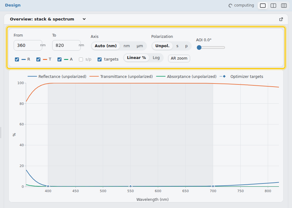
The layers panel is on the left and one or more panes are in the center, each showing one view; the overview pane holds the spectrum. The spectrum's bar holds the range, axis unit, polarization, angle of incidence, the R / T / A curves, s/p split, targets, linear or log scale and AR zoom. The axis unit Auto shows nm when the reference wavelength is below 1000 nm and µm from 1000 nm up; nm or µm can be chosen instead. Wavenumbers (cm⁻¹) are accepted when importing measured spectra and n,k data, and converted to wavelength. Spectrum plots keep physical limits: R, T and A stay within 0–100 % (10⁻¹⁵ to 1 on the log scale) and the wavelength within the computed range, at any zoom or pan. A sweep runs anywhere from 50 nm to 100 µm (3 THz) with up to 6,001 points; the reference and field wavelengths cover the same range and a layer can be up to 200 µm thick.
Terahertz. A design with a terahertz film, a coating layer of measured \(n\), \(k\) data reaching past 100 µm, reaches 3 mm (0.1 THz) and 2 mm layers. Past 100 µm only measured data is used: custom constant, Cauchy and Sellmeier materials hold to 100 µm, so a THz film is a library material tagged THz or your own measured table. The THz library, all used only inside their data: vacuum-deposited films of Ta\(_2\)O\(_5\) (sputtered, 0.5 µm–1 mm; e-beam, to 400 µm), HfO\(_2\) (sputtered, to 500 µm), Al\(_2\)O\(_3\) (PEALD, to 993 µm; e-beam, to 125 µm), MgF\(_2\) and TiO\(_2\) (e-beam and ALD, to 125 µm); substrates of float-zone silicon (to 310 µm), undoped GaAs (to 400 µm), CVD diamond (to 500 µm), HDPE and TPX (to 200 µm). Doped wafers' free carriers are not in the silicon data. Beyond a material's data the spectrum is blank.
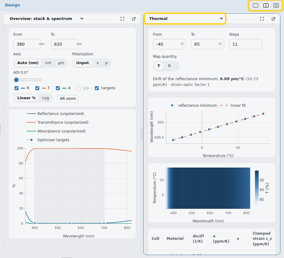
Design's pane menu lists its own views and, under Analyze, the Angle map, Phase & GDD, Ellipsometry and Ultrafast & NLO.
| View | Shows |
|---|---|
| Spectrum | The spectrum's finer settings and results: metrics and color, points, focused-beam cone averaging, air path, spectrophotometer slit, color illuminant; the band table; pinned reference curves; measured spectra; CSV export. Click the spectrum to pick the wavelength for the field views. |
| Angle map | R, T or A over wavelength and angle of incidence. |
| Index & E-field | The refractive-index profile through the stack and the standing-wave field intensity \(|E|^2\), which matters for laser damage. |
| Admittance | Macleod's admittance diagram with iso-reflectance circles. |
| Phase & GDD | Reflected and transmitted phase, group delay, GDD and third-order dispersion (TOD), plus the ellipsometric angles \(\Psi\) and \(\Delta\) at the chosen angle of incidence. |
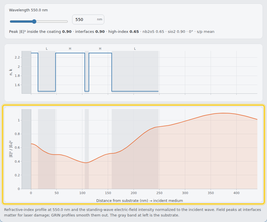
Laser damage estimate. Under the field, Laser damage estimate (femtosecond pulses) gives each film
material's single-pulse threshold from its band gap, by the scaling of Mero et al. (Phys. Rev. B 71, 115109; Opt. Eng. 44, 051107;
2005), \(F_\mathrm{int} = (0.074\,E_g - 0.16)\,\tau^{0.30}\) J/cm² with \(\tau\) in fs, divided by the peak \(|E|^2/|E_0|^2\) in that
material at the field wavelength. The lowest is the coating's estimate and names the limiting material. Band gaps are representative
film values (Mero's for TiO₂, Ta₂O₅, HfO₂, Al₂O₃, SiO₂); replace them with measured values. The fit is for 800 nm, about 25 fs to 1 ps and
3.3–8.3 eV; outside that the estimate is flagged. It does not cover multi-pulse (incubation), defect-driven or nanosecond damage
(POST /api/ldt).
Field targets. An E2 target bounds the peak \(|E|^2/|E_0|^2\) at its wavelength, usually with \(\le\) next to the reflectance targets of an HR: in the whole coating, at its interfaces (the layer boundaries), at its layers' centers (each layer's mid-depth) or in its high-index layers. Outer layers limits it to the outermost layers from the incident side (with their lower boundary), where a mirror's standing-wave field peaks; 0 counts every layer. The field is the nominal design's, rough interfaces included. Local and global optimization, needle (every strategy) and synthesis take field targets; needle solves the field of every candidate stack, so such runs are several times slower.
Axis. Show the spectrum in nm, µm or wavenumbers (cm⁻¹). The sweep limits and target bands are then entered in the same unit. The wavenumber axis runs from high to low, as in FTIR spectra. Designs are stored and calculated in nm, and the setting is remembered per browser.
Measured data. Measured data… opens a window where you can drop a file, browse for one, or paste text or CSV. It reads a wavelength column and one or more R, T or absorbance columns, in % or fractions, with the unit (nm, µm, Å, eV, cm⁻¹) from the header. Cary/Lambda paired-column exports load one curve per sample; absorbance is converted to \(T = 10^{-A}\). Excel workbooks (.xlsx), JCAMP-DX files (plain or compressed), UTF-16 text and files that write decimal commas (1,5) load too; the legacy .xls and the instruments' binary formats do not (save as .xlsx or CSV). Each measured curve is drawn dotted in its quantity's color. The list under the plot shows the RMS difference from the calculated curve where both exist. To fit a design to the data, use Fit measured data.
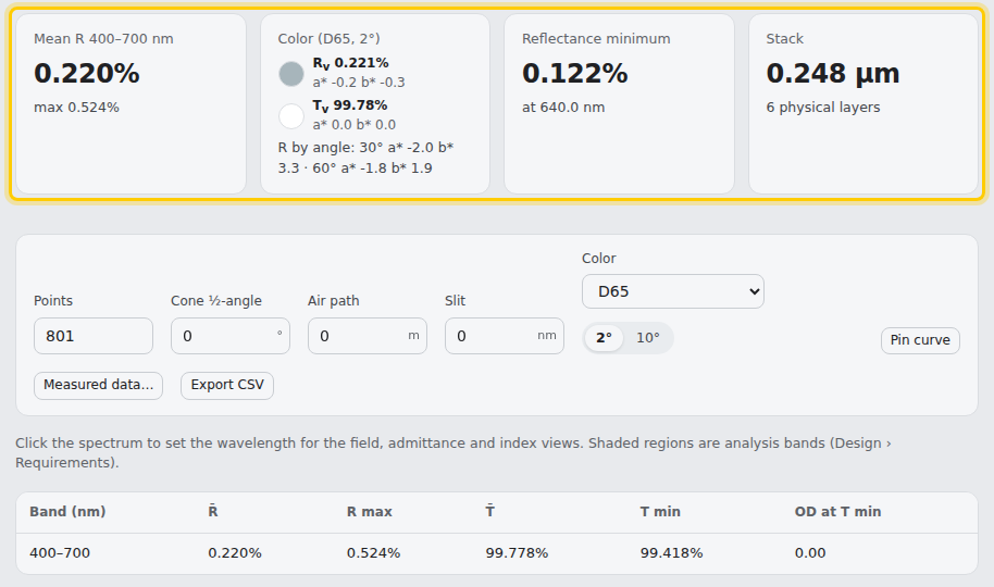
The metric cards summarize the design: band-averaged R or T, optical density, pass- or stop-band center and width, 50 % edges, reflected and transmitted color (CIE 1931, luminous \(R_v\) and \(T_v\)), and total thickness.
Under the spectrum, Color difference, dominant wavelength, purity, yellowness, CCT, chromaticity diagram gives, for the reflected and the transmitted color: L*a*b*, \(Y\), dominant (or complementary) wavelength, excitation purity, ASTM E313 yellowness, the light's correlated color temperature and \(D_{uv}\) (the illuminant as the source; Ohno, LEUKOS 10, 47, 2014: nearest blackbody on a 1 % table, refined by a triangle or a parabola; none more than 0.05 from the Planckian locus), and \(\Delta E\) (CIEDE2000, CIE94, CMC or CIE76) from a reference color. The diagram shows CIE 1976 u′v′, CIE 1931 xy or CIELAB a*b* with the spectral and Planckian loci, the white point and the reflected color's path from 0° to 60°. CRI is not computed (it needs the CIE test-color samples).
Temperature
Set an operating temperature in the editor, or open the Thermal view for a sweep. For each temperature:
The rest of this section is for members
Create a free account to read the full documentation: production, monitoring, optimization, the APIs and the physics.
Stress & bow
The Stress & bow view sweeps from any temperature down to 4 K (presets: lab, MIL, LN₂ 77 K, LHe 4 K). Each film carries its growth stress plus the thermal mismatch accumulated since deposition, using the integrated strains above:
The rest of this section is for members
Create a free account to read the full documentation: production, monitoring, optimization, the APIs and the physics.
History & CI
With a PostgreSQL database configured (DATABASE_URL), press Ctrl+S (File › Save) anywhere to commit the working design with an optional message.
Committing needs an account (email and password); you see only your own designs and those shared with you. Every commit stores the full design, sweep, bands and targets plus key parameters (substrate, layer count, thickness, materials, spec band, band R/T),
then runs a four-gate pipeline in the background:
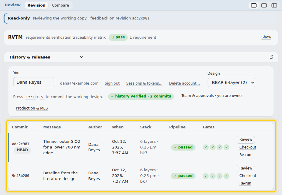
- Layer design: layer count, thinnest layer, total thickness, absorption;
- R/T vs spec: every target band (\(\le\) and \(\ge\) are hard limits; \(=\) targets are ideals judged within ±1 %);
- Stress & bow: bow in waves at 20 °C and over the operating range (to 4 K), peak tensile stress (crazing risk), spectral drift;
- Manufacturability: SPC Monte-Carlo yield, monitoring terminations near turning points, deposition time.
The header chip shows HEAD and its pipeline status; ● marks uncommitted edits. Review › History & releases (a view in the Review tab; the header chip and History, gates and releases… in Review's side bar open it) lists commits with per-gate results, the parameter diff from the parent, Review (show the commit read-only in Review), Checkout (load it into the editor) and Re-run.
Each commit is named by a hash that covers its content and its parent's hash, so any edit to history is detectable. The tab re-checks the whole chain and shows history verified, or history altered with the commits affected.
Signing in. Forgot password? in the sign-in dialog emails a code that sets a new password (when the server sends email). On Pro and Team, Settings › Account › Two-step sign-in also asks for a code after the password: from an authenticator app (scan the QR code) or emailed to you. Turning it on gives ten recovery codes, each valid for one sign-in if the phone or mailbox is lost; store them securely. Remember this device skips the code on that browser for 30 days (your password is still needed); Forget them in the same settings, or a password reset, ends that. A site administrator can turn two-step sign-in off for you. Accounts that use single sign-on get two-step sign-in from their identity provider instead.
Each revision also keeps a design record: the complete data behind its results: every material's dispersion model with its tabulated n,k and source-file checksums, the thermal-expansion and mechanical constants, n and k on the design's wavelength grid, the reference spectrum and the solver version. Pipeline runs and re-runs of a revision always use its record, so later changes to the material library never change an old revision. Reproduce re-evaluates the revision from its record and lists anything that has changed in the library since. Download audit package gives a ZIP of readable files (JSON and CSV) with SHA-256 checksums.
Review & RVTM
The Review tab is read-only: inputs are frozen and edits refused, while plots and analysis stay live (collaborators see every tab this way). It has two parts, switched at the top of the center: Revision reviews one revision, and Compare puts up to four side by side (below).
Revision shows the working copy until you pick a saved revision in the side bar: a release tag of any design you can read, each design's latest revision, or any commit of a chosen design (or Review on a row of History & releases). Picking one leaves the working copy untouched; Review the working copy returns to it. Check out to edit loads the revision into the editor and opens Design. At the top sits the RVTM, the requirements verification traceability matrix: one row per requirement (each spec target, the bow and film-stress limits of the mechanical requirement, and the deposition temperature and time of the thermal budget) with its limit, how it is verified, the evidence plot, the predicted value, the margin and pass / fail, judged exactly as the pipeline gates judge them. Under every plot, and on every RVTM row, reviewers can tick Reviewed, react with 👍 👎 ❓ ⚠️ and leave comments. Feedback belongs to the saved revision being viewed, and everyone the design is shared with can give it. Feedback is informal; the release signature is the formal approval. Comments cannot be edited or deleted. In Review › Revision the bottom bar gathers the revision's feedback: every plot and RVTM row that has a mark or a comment, with its latest comment; clicking one shows it.
Comparing revisions
Review › Compare puts up to four revisions side by side. The side
bar picks them: the working copy, any release tag (a release candidate such as B-RC1, or a released
Rev A) of any design you can read, each design's latest revision, or any commit of a chosen design. One of them is the
baseline. The center shows one RVTM across all of them, a column per revision with its prediction, margin and
pass / fail, and the largest clear margin on a row starred. Baseline's spec judges every revision against
the baseline's requirements (its spec targets, mechanical requirement and thermal budget); Each its own judges each against
the requirements it was saved with, and a revision without a requirement shows not required. Under it, 1, 2 or
2 × 2 plots overlay the revisions, each plot showing one of R, T, A, optical density, R on a log scale, ΔR or ΔT against
the baseline, or reflected phase, GD and GDD. All revisions are computed on one sweep: the working copy's settings with the
range, angle and polarization set in the side bar. The picks and plot settings are kept in the browser. The center
stays empty until two or more revisions are picked and at least one of them is saved: a working copy alone has nothing to
compare against.
Example: from 5 to 6 layers
One design change taken through Optimize, History and Review: a 5-layer visible AR that misses its spec at the blue edge, a
sixth layer added, and the two revisions compared. scripts/layer_upgrade_example.py reproduces every number and
scripts/docs_case_5to6.js the figures. The optimizer is time-limited, so a rerun can move a thickness by a few
tenths of a nanometer.
Setup
- Design: Library › 6-layer VIS BBAR (Nb2O5/SiO2) with its first cell, the Nb2O5 at the substrate, deleted: L H L H L on N-BK7 in air.
- Requirements (Overview side bar), R at 0°, unpolarized, over 400–700 nm: the preset's R = 0 as the design aim (RVTM status goal), R ≤ 0.25 % with Band: mean in the target's options, and R ≤ 0.55 % at every sample. The two limits have weight 4.
- Optimize: Multi-start, 24 starts, 40 s; Min thickness 8 nm (the library design's manufacturability floor), Max thickness 150 nm.
Revision A: five layers
Multi-start with Jump σ 60 % gives 69.42 / 12.68 / 38.64 / 115.30 / 87.07 nm, SiO2 first, 323.1 nm in all (the default 20 % jumps stay in a poor minimum, R max 1.7 %). Save it. In the RVTM the mean, 0.196 %, passes with 0.054 pp to spare; R max, 0.567 % at 400 nm, fails by 0.017 pp.
Revision B: a sixth layer
In Layers, + Layer adds a cell at the air side: make it Nb2O5, 10 nm, and drag it by its row number to row 1, next to the substrate. Optimize again (Jump σ back to 20 %). It converges to 13.65 / 34.14 / 56.92 / 8.00 / 44.42 / 90.97 nm, the library design to within 0.01 nm, 248.1 nm in all. Save it.
Keep the floor. With Min thickness 0 the optimizer shrinks the new layer to 0.48 nm and lands back on revision A (R max 0.566 %). The 6-layer solution is a different family; the 8 nm floor is what makes the optimizer find it.
What changed: the version history
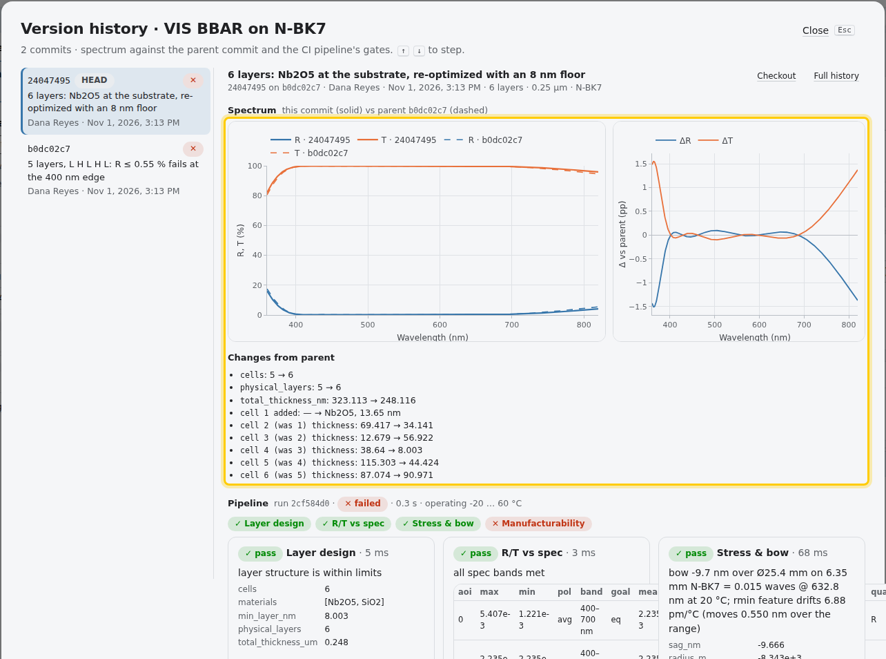
In Review › History & releases, click B's message. The version history shows B's R and T against A's (dashed), ΔR and ΔT,
and Changes from parent. The diff aligns the two stacks on their layer sequence, so the inserted layer is one line,
cell 1 added: Nb2O5, 13.65 nm, and every layer above it is listed under its new number and its old one,
cell 2 (was 1) thickness: 69.417 → 34.141. Every thickness moved: the sixth layer re-balances the whole stack, it
does not just add to it. The Δ plot spans the design's sweep, 360–820 nm; outside the band B departs from A by up to
1.5 pp.
Side by side: Review › Compare
Pick both revisions in the side bar, A as the baseline, judged on Baseline's spec. The RVTM comparison puts the verdicts next to each other and stars the larger margin on each row; Values lists the figures and colors:
| A, 5 layers | B, 6 layers | |
|---|---|---|
| Total thickness | 323.1 nm | 248.1 nm |
| R mean ≤ 0.25 % | 0.196 %, pass ★ | 0.224 %, pass |
| R ≤ 0.55 % | 0.567 % at 400 nm, fail | 0.541 % at 400 nm, pass ★ |
| R min | 0.06 % at 644 nm | 0.12 % at 640 nm |
| Reflected color L*, a*, b* (D65, 2°) | 1.8, 0.4, −0.6 | 2.0, −0.3, −0.3; ΔE*ab 0.75 |
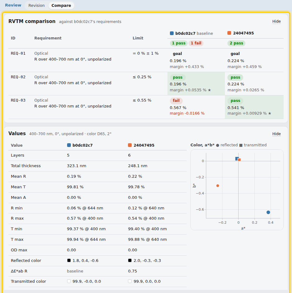
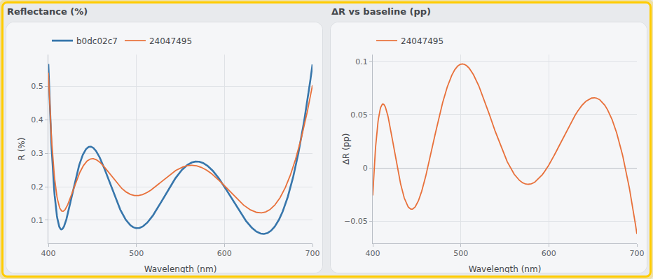
The plots show what the sixth layer traded. ΔR against A is positive over 69 % of the band, up to +0.098 pp near 500 nm, and negative around 440 and 575 nm and at both edges: −0.026 pp at 400 nm, where the spec was failing, and −0.062 pp at 700 nm. B's mean is 0.028 pp higher, still inside the 0.25 % limit. The 5-layer design had the better average but could not hold the blue edge.
What the pipeline says
Each save runs the CI pipeline. Both revisions pass Layer design, R/T vs spec and Stress & bow, and both fail Manufacturability. Its Monte Carlo (200 runs; 1 % random error per layer, 0.5 % tooling per material, index σ 0.003) predicts a yield of 2 % for A and 19 % for B, against 90 % to pass. The mean limit holds (99.5 % and 86 % of runs meet it); the 0.55 % edge does not (2 % and 21.5 %), because B meets it by only 0.009 pp on paper. The sixth layer gives the better design: thinner, inside the spec, nearly ten times the yield. It does not yet give a releasable one. The next step is margin at the edge: Robust optimization (Optimize, thickness σ), a design limit tighter than the spec, or a renegotiated R max.
Releases & signatures
A design goes to production through a release: a reviewed, signed revision with a label (Rev A, B, …). The workflow is built for design-control requirements such as AS9100 §8.3 (design review, outputs and changes).
The rest of this section is for members
Create a free account to read the full documentation: production, monitoring, optimization, the APIs and the physics.
Lifecycle, qualification & NCRs
Every design is in one stage: design (simulation only), prototype or production. Lifecycle in Review › History & releases shows the stage, what the next one needs, qualifications, and the log of every change (who, when, why).
The rest of this section is for members
Create a free account to read the full documentation: production, monitoring, optimization, the APIs and the physics.
Material experiments
An experiment gets verified \(n, k\) data for a substrate or a film. It asks the process, tool and metrology engineers for N measurements of a substrate, or N test depositions of a single film (YbF₃, 50 nm on Si, in a given chamber and process), averages their results, checks them against the limits you set, and once verified publishes the average to a material library. An experiment can stand alone, or be part of a design's qualification and hold up its production until the data is verified. Production › Experiments lists the experiments you can see (all, the ones with a task for you, or the open design's) beside the open one.
The rest of this section is for members
Create a free account to read the full documentation: production, monitoring, optimization, the APIs and the physics.
Production & MES
A manufacturing execution system (MES) connects in both directions. Thin Film Forge tells it when a revision is released, it pulls the controlled run sheet, and after each coating run it posts the measured spectra back. Each run is judged against the released spec and charted here. Runs & SPC in Review › History & releases shows the runs, their verdicts and the control charts, and lets the owner manage webhooks.
The rest of this section is for members
Create a free account to read the full documentation: production, monitoring, optimization, the APIs and the physics.
Notifications & Slack
Thin Film Forge emails people when something needs them or concerns their work, and, where your site connects Slack or Mattermost,
messages them there too. Nobody is told about what they did themselves. In Slack you can also ask the /tff bot what is
waiting for you.
The rest of this section is for members
Create a free account to read the full documentation: production, monitoring, optimization, the APIs and the physics.
PLM
A design can be linked to a document or item that already exists in PTC Windchill, Siemens Teamcenter or Arena
(one system per installation, set by the administrator). Thin Film Forge never creates PLM objects.
Push sends a saved revision: the object's main file is replaced by the monolithic EIDP (the end item
data package and the coating datasheet in one bookmarked PDF), and the datasheet and the revision's audit package
are added beside it. The check-in note carries the revision's TFF version (TFF-<design>-<release>),
commit hash and record SHA-256. With auto export on,
every signed release is pushed automatically. Pull fetches the object's requirements, proposes spec targets
from sentences such as R ≤ 0.5 % 430–670 nm at 45°, and stores the snapshot tagged with the revision it was
pulled against; targets are applied by hand after review.
The rest of this section is for members
Create a free account to read the full documentation: production, monitoring, optimization, the APIs and the physics.
Ultrafast & nonlinear optics
Pulse through the coating
A Gaussian pulse (center wavelength, FWHM duration, optional input chirp) is sent through the coating's actual complex reflection or transmission spectrum for any number of bounces, plus an optional length of bulk material, by FFT. Outputs: duration and its transform limit, added GDD and TOD, the fraction of peak power kept, the temporal intensity, the instantaneous-frequency chirp, and the output spectrum and spectral phase.
The rest of this section is for members
Create a free account to read the full documentation: production, monitoring, optimization, the APIs and the physics.
Ellipsometry
The Ellipsometry tab computes what a spectroscopic ellipsometer measures on the loaded design, at several angles at once: \(\Psi\) and \(\Delta\), \(N\), \(C\), \(S\), the full normalized Mueller matrix, and the depolarization.
The rest of this section is for members
Create a free account to read the full documentation: production, monitoring, optimization, the APIs and the physics.
Optimize & needle
The rest of this section is for members
Create a free account to read the full documentation: production, monitoring, optimization, the APIs and the physics.
Synthesize
Start from constraints instead of a design (File › New film… › Synthesize). Choose the substrate, the incident medium, the coating materials you can deposit, the maximum number of layers, thickness limits and the R/T specification over one or more wavelength ranges.
The rest of this section is for members
Create a free account to read the full documentation: production, monitoring, optimization, the APIs and the physics.
Fit measured data
After a coating run, fit the loaded design to the measurement to estimate what was deposited.
The rest of this section is for members
Create a free account to read the full documentation: production, monitoring, optimization, the APIs and the physics.
Characterize a film
The Characterize tab finds the optical constants \(n(\lambda)\), \(k(\lambda)\) and thickness of a single film (or a substrate) from any mix of ellipsometric \(\Psi/\Delta\) at several angles and photometric \(R/T\) spectra.
The rest of this section is for members
Create a free account to read the full documentation: production, monitoring, optimization, the APIs and the physics.
Optical monitoring
The Monitoring tab simulates direct optical monitoring on the part: the transmission or reflection each layer produces as it grows on top of the layers already deposited. For every layer it reports the monitor wavelength, the start and stop signal, the turning points passed, and the signal slope at the stop point.
The rest of this section is for members
Create a free account to read the full documentation: production, monitoring, optimization, the APIs and the physics.
Inline re-optimization
The Re-optimization tab (Production) closes the loop between the optical monitor and the design during a run. After each layer it estimates the thicknesses actually deposited from the monitor readings, tells you when to stop the layer in progress, and re-optimizes the remaining layers when the finished part would miss its targets. OTF Studio sells the same idea as taReo. It works with two kinds of monitor, chosen under Monitor: Broadband (a spectrometer) or Single λ (a monochromator). They take different readings and give different results; choose the one your coater has.
The rest of this section is for members
Create a free account to read the full documentation: production, monitoring, optimization, the APIs and the physics.
Re-optimization examples
Four runs on library designs, each answering one practical question. The readings are synthetic (Production ›
Re-optimization › Synthetic reading, or POST /api/reopt/scan), with a known error put in, so each estimate can be checked
against the truth. scripts/reopt_examples.py reproduces every number. Merit is the RMS deviation from the
Requirements targets, as Optimize reports it; re-optimization starts when the predicted part is 20 % worse than planned (the
default).
The rest of this section is for members
Create a free account to read the full documentation: production, monitoring, optimization, the APIs and the physics.
Run sheets & controller export
The Run sheet tab turns the design into the per-layer table a coater loads into its deposition controller.
The rest of this section is for members
Create a free account to read the full documentation: production, monitoring, optimization, the APIs and the physics.
Worst case & sensitivity
Production › Worst case answers whether a run can fail anywhere inside stated tolerance bounds, and which tolerance to tighten if so. (SPC answers how often a run meets spec.)
The rest of this section is for members
Create a free account to read the full documentation: production, monitoring, optimization, the APIs and the physics.
SPC & yield
Estimate how many coating runs will meet spec before you build.
The rest of this section is for members
Create a free account to read the full documentation: production, monitoring, optimization, the APIs and the physics.
Production case studies
How four library designs hold up to the thickness errors of different deposition processes. Each design is run
through the SPC Monte Carlo (400 runs, fixed seed) with thickness errors only: index σ 0 and no monitor drift, so the
numbers isolate what the thickness control does. scripts/production_cases.py reproduces every number;
with 400 runs a yield's standard error is at most 2.5 points. The specs are each design's nominal performance plus a
margin a customer might accept; a design's own Requirements are optimization targets, which none of these meets as
built.
| Design (library) | Layers | Thinnest | Acceptance spec (nominal) |
|---|---|---|---|
| 6-layer VIS BBAR | 6, 248 nm | 8.0 nm | R mean ≤ 0.3 % (0.222) and R ≤ 0.8 % (0.541), 400–700 nm |
| Quarter-wave HR @ 1064 | 25, 3980 nm | 137.0 nm | R ≥ 99.0 % (99.348), 1000–1130 nm, out to the stop band's shoulders |
| Green broad band-pass | 54, 4709 nm | 28.9 nm | T mean ≥ 95 % 515–585 nm (97.21); T ≤ 2 % 400–470 nm (0.92); T ≤ 10 % 640–780 nm (5.30) |
| Hot mirror | 48, 4292 nm | 5.0 nm | T mean ≥ 80 % 450–650 nm (84.78); T ≤ 10 % 760–1100 nm (6.59) |
Relative or absolute thickness error
A crystal- or time-controlled process makes errors that scale with the layer (relative, σ in %); an optical or end-point monitor stops each layer with an error of about the same size whatever its thickness (absolute, σ in nm). Yield, in %, with each kind alone, every layer drawn independently:
| Relative σ (%) | Absolute σ (nm) | ||||||||||
|---|---|---|---|---|---|---|---|---|---|---|---|
| Design | 0.1 | 0.25 | 0.5 | 1 | 2 | 0.05 | 0.1 | 0.25 | 0.5 | 1 | 2 |
| BBAR | 100 | 100 | 99.5 | 90.0 | 70.0 | 100 | 100 | 98.0 | 82.0 | 55.2 | 13.8 |
| HR 1064 | 100 | 100 | 100 | 100 | 95.0 | 100 | 100 | 100 | 100 | 100 | 99.0 |
| Green band-pass | 100 | 98.5 | 95.2 | 77.2 | 22.0 | 100 | 100 | 98.8 | 93.5 | 83.5 | 32.8 |
| Hot mirror | 100 | 100 | 100 | 99.8 | 94.5 | 100 | 100 | 100 | 100 | 99.5 | 92.5 |
- Thin layers make absolute error the risk. The BBAR's 8 nm layer takes a 0.5 nm error as 6 % of itself: 82 % yield, where 0.5 % relative error keeps 99.5 %. At 1 nm against 1 %, 55 % against 90 %.
- Many thick layers make relative error the risk. The band-pass's 54 layers, 29–117 nm, shift its edges with every percent: 77 % yield at 1 % relative, 94 % at 0.5 nm absolute.
- Random errors average out in a periodic stack. The HR's 25 quarter-waves keep 100 % to 1 % relative and 1 nm absolute: independent per-layer errors scatter about the design and barely move the stop band. Correlated errors move it (next).
Deposition processes
Three process profiles from what is published, a "±" figure read as 2σ:
| Process | Model (1σ) | From | BBAR | HR 1064 | Band-pass | Hot mirror |
|---|---|---|---|---|---|---|
| E-beam evaporation, crystal control | 1 % per layer, 0.5 % per material (tooling) | ±2 % thickness, the acceptance in the built-in chambers' qualification plan; no vendor figure found. Tooling: the app's default | 88.5 | 93.8 | 79.0 | 99.5 |
| Magnetron sputtering, optical monitoring | 0.1 % per layer, 0.1 % per material | ±0.2 % layer thickness run to run, Bühler HELIOS brochure; taken for both terms | 100 | 100 | 100 | 100 |
| Ion beam sputtering | 0.05 nm per layer | < 0.1 nm thickness control, Veeco SPECTOR, per an Edmund Optics press release | 100 | 100 | 100 | 100 |
The evaporation profile costs the HR 6 points although 1 % random error alone costs it none: the 0.5 % tooling error is shared by every layer of a material, so it shifts the whole stop band and its shoulders leave the spec band. The band-pass loses most to its 400–470 nm blocking limit (81.5 % of runs meet it). Both sputtering profiles hold every design at 100 %: at these error levels the design, not the process, sets the yield.
Across the fixture
The Monte Carlo above is one position in the chamber. Thickness also varies across the fixture; the script scales the nominal design by 1 ± the fixture's uniformity and checks the parts at the edge:
| Fixture uniformity | BBAR | HR 1064 | Band-pass | Hot mirror |
|---|---|---|---|---|
| ±1 %, evaporation calotte (built-in chamber) | thick edge fails | thick edge fails | thick edge fails | pass |
| ±0.5 %, HELIOS brochure; IBS planetary (built-in chamber) | pass | pass | pass | pass |
A part at the thick edge of a ±1 % calotte fails three of the four specs before any run-to-run error: a whole-stack scale moves every edge together. With such a fixture, the uniformity budget, not the layer control, decides the yield; masking, a planetary fixture or a spec with room for a 1 % shift are the levers. For a fitted fixture model (thickness and index by position) and net yield over the parts, record site-tagged runs and use Production › SPC / yield with the chamber's uniformity model.
Caveats
- The vendor numbers are published claims without test conditions (substrate size, material, position, measurement method). Ask the vendor for the datasheet behind them before you rely on them.
- Index errors are left out on purpose. With the default index σ of 0.003, all yields come out lower; set your own in Production's side bar (Process error model) and run Production › SPC / yield.
Physics & conventions
Isotropic stacks are solved with the characteristic-matrix (Abelès) method in Macleod's convention, \(N = n - ik\) (materials are entered as \(n + ik\) with \(k \ge 0\) and conjugated on entry). For layers \(r = 1 \ldots q\) on a substrate \(m\):
The rest of this section is for members
Create a free account to read the full documentation: production, monitoring, optimization, the APIs and the physics.
Validation
The solver is tested against closed-form results (Fresnel, Brewster, quarter-wave AR and mirror formulas, total internal reflection, incoherent rear surface) and against an independent transfer-matrix implementation for absorbing, oblique s and p stacks.
Fourteen designs are cross-checked against two independent transfer-matrix codes, tmm (Byrnes) and PyMoosh (Langevin et al.,
JOSA B 2024), all fed identical per-layer indices. They cover a single-layer AR, a 45° broadband AR, a 25-layer mirror with its standing-wave
field, a 1,820-layer rugate down to OD 3.7, a two-cavity band-pass with its group delay, absorbing silver and aluminum stacks with the
absorption in each layer, a 69-layer ppm-level GaAs/AlGaAs mirror, a germanium IR AR with absorbing films, a thick incoherent substrate,
and in the infrared and terahertz a 4.26 µm CO₂ band-pass with an absorbing Ge-film cavity, a ZnS/Ge long-wave pass, a 10.6 µm ZnSe
window with an incoherent rear face, and a 150 µm silicon etalon with lossy parylene AR from 0.3 to 3 THz.
\(R\), \(T\) and \(A\) agree to better than \(10^{-13}\) in every case.
It is also checked against designs published in Optica, JOSA B, IEEE and Applied Optics papers. The Validation tab in the app shows the quoted design, assumptions, computed and published values for each:
| Design | Published | Thin Film Forge |
|---|---|---|
| GaAs/AlGaAs mirror, 34.5 periods, 4.5 µm (Optica 2021) | \(T = 140\) ppm | 141.6 ppm |
| GaAs/AlGaAs, 38.5 / 41.5 periods, 1550 nm (Optica 2016) | 10 / 5 ppm | 10.4 / 4.4 ppm |
| GaAs/AlGaAs, 35.5 periods, 1064 nm (JOSA B 2019) | 10 ppm | 8.6 ppm |
| Cryolite/ZnSe omnidirectional mirror (IEEE JLT 1999) | 604.3–638.4 nm | 606.6–643.0 nm |
| Optimal SiO₂/Si omnidirectional lattice (IEEE JLT 1999) | \(\eta = 0.324\), center 0.275, 25 % | 0.328, 0.2744, 25 % |
| Band-pass thermal drift vs substrate CTE (Applied Optics 1995) | +0.018 → −0.005 nm/°C | between the model limits |
Files & sharing
| Action | Result |
|---|---|
| File › Export › Design (JSON), File › Open file | A JSON file with the design, sweep, bands and targets, including custom materials. |
| File › Import design | A design from another program: an OpenFilters project, or the layer table that
Essential Macleod, TFCalc, OptiLayer, FilmStar or a spreadsheet copies or exports as text (tab, comma,
semicolon or space separated). The header names the columns: material, physical thickness (nm, µm, Å) or optical
thickness (QWOT, FWOT), and optionally n and k. Optical thicknesses are converted with the file's own index when it
has one, so the physical thicknesses match the other program. Medium and substrate rows fix the order; without them
the first row is taken as next to the substrate, and the preview lets you flip it. Materials are matched to the
library by id, name, formula and common aliases (SiO2 is the SiO2 film as a layer and fused silica as a
substrate); a material the library lacks becomes a constant n, k from the file (no dispersion) or is left to map by
hand. Where the file's index differs from the library's by more than 0.02 at λ₀ the preview says so. Binary
design files are not read: export them as text first. |
| File › Export › Layer table (CSV) | Every physical layer after repeats and GRIN discretization, with its index at the reference wavelength. |
| File › Export › Spectrum (CSV) | \(R\), \(T\), \(A\) for unpolarized, s and p light, plus reflected phase and group delay. |
| File › Export › Datasheet (PDF) | The coating datasheet of the design as it stands: construction summary, the spectrum with the spec bands drawn (dashed curves for the other angles and polarizations the spec names; an OD panel when it has OD bands), the spec table judged exactly as the pipeline's optics gate judges it, CIE color when the sweep covers 380–780 nm, and the physical layer table (material, thickness, QWOT, n, k at λ₀; front and rear; the first 2 000 layers). Vector PDF with embedded fonts. |
| File › Export › Datasheet (Excel) | The same content as a workbook: Summary, Specification, Layers (every layer) and the spectrum (R, T, A unpolarized, s and p) as numbers, one sheet each. |
| File › Export › Datasheet (Word) | The datasheet as an editable .docx: construction, the spectrum plot, the specification and the layer table. |
| File › Export › Spectrum (SVG) | The datasheet's spectrum plot with the spec bands as a vector SVG (text kept as text) for slides and documents. |
| File › Export › Datasheet of HEAD (PDF) | The same for the saved HEAD revision, computed from its design record (frozen n, k and models), with a revision page: commit and record hashes, pipeline gates, and each release with its signatures and whether the signature chain verifies. |
| File › Export › EIDP report (PDF)… | An end item data package. The cover carries the identifying data
(document number and revision, project, customer, part numbers, PO, serial/lot, substrate, date, design revision),
a compliance verdict and a prepared/checked/approved signature block. After it come a design summary, the requirements
verification traceability matrix (spec value, design value, margin and PASS / FAIL, judged like the pipeline's
gates), the plots you list and the layer table. Each plot is a spectrum, OD, phase/GD/GDD, E-field or bow vs
temperature, with its own range, angles, polarizations, axis limits, title and caption. Generate it from the design
as it stands or from the saved HEAD revision, which adds the revision record. Save config writes the
settings as JSON; the same file drives POST /api/report/eidp and
python -m thinfilm.eidp design.json config.json -o report.pdf. The Report tab builds the same
report live: its settings in the side bar, the PDF preview in the pane, rebuilt a moment after each change.
A report whose text (cover fields, notes, plot titles and captions, design and material names, the revision
record) holds offensive language is not generated; the error names the field to edit. |
| File › Export › Audit package | The design record of the saved HEAD revision (see History & CI). |
| File › Export › Copy share link | A link that opens the current design and sweep. |
Workspace
Workspace (in the menu under your user icon, top right) shows your roots: Private, your team's (see Folders, projects and teams) and Shared with me. Each folder and project holds designs and files (measured spectra, n,k tables, reports, exports, anything). A Private root holds 50 MB; a team root 50 MB per engineer seat, shared by the team; the side bar shows the open root's use. Upload or drop files from your computer onto the list or onto a folder, make folders and projects, rename (F2), move (drag onto a folder in the list, the tree or the path, or Move to…: designs and files to another root, folders within theirs), duplicate, download and delete (Delete; a folder goes with the files in it, there is no trash, and a folder holding a design is not deleted). Double-click a design to open its latest revision in Design. Click a column header to sort; Filter everything searches every root. Images and text files (CSV, JSON, plain text) preview beside the list. Share sets who sees a folder and its members; Team tags (the team's lead) tags members. Save design saves the working copy as a new tracked design in the open folder (Save as; File › Save as picks the folder too), Export JSON writes it as a design JSON file there, and Open as design opens such a file as the working copy. In a team folder reviewers read the files and engineers change them. A file of a name the folder already has asks whether to replace it, keep both or skip. Files are served only as downloads or as plain previews: an uploaded HTML or SVG file never runs as a page.
Terminal
The terminal is in the bottom bar of Design (and, with the terminal button in its header, of every other bottom bar). It builds
and edits the open design from the keyboard. Commands start with --; several can share a line, run in order, and stop
at the first error. Every edit goes through the same path as the editor, so Undo works, a read-only design refuses
edits, and the plots follow. Tab completes a command or a material name, ↑ ↓ recall earlier lines,
Ctrl+L clears the screen, and help lists the commands.
| Command | Does |
|---|---|
--create [name] | A new film: no layers, air over a BK7 substrate. When a design with layers is open it asks Replace … with a new film? [y/N] first; anything but y cancels the rest of the line. |
--sub <material> [--inc m] [--exit m] [--mm t] [--back on|off] | The substrate, by name. The incident and exit media are air unless
--inc / --exit name others; --mm is the substrate thickness in mm; --back on turns on the rear-face coating. |
--new <material> <qwot> (-n) | Adds a layer on the air side. The thickness is in quarter-waves at the reference wavelength:
-n YbF3 1.5 is 1.5 QWOT, 136.3 nm at 550 nm. |
--lrange <low> <high> [unit] | The graph limits. The unit is nm by default, or um, cm-1, THz; the ends may come in either order. |
ps | Prints the stack: number, material, nm and QWOT, layer 1 next to the substrate. |
--del n, --set n qwot | Removes layer n; sets its thickness in QWOT. |
--ref nm, --aoi deg, --pol s|p|avg | The reference wavelength (the QWOT basis), and the angle and polarization of the plots. |
--opt [global|local|multistart] [thickness|index|both] [--min nm] [--max nm] [--time s] | Optimizes against the
Requirements. The default is global, thickness only, layers 0–1000 nm, up to 30 s, as the Optimize tab starts. The result is applied as an
edit and the merit before and after is printed; --undo reverts it. Needle runs as a background job: use the Optimize tab. |
--undo, --redo | Steps through edits. |
--materials [filter] | Lists library materials with their category and data range. |
tui | The stack editor, below. |
Materials are matched by id or name, ignoring case and hyphens (bk7, N-BK7); a miss suggests close names.
A quarter-wave AR on glass, graphed over the visible:
--create AR test --sub BK7 -n MgF2 1 --lrange 400 700
ps
A new film has no targets, so --opt needs some first (Overview › Requirements, or a library design that has them). With the library's
6-layer VIS BBAR open, --opt local both --min 8 --max 150 lowers its merit from 2.65·10−4 to 1.24·10−4 by also varying the indices.
The stack editor
tui replaces the prompt with the stack, which follows the design as it changes. ↑ ↓ pick a layer (the top row
is the air side); ← → change its QWOT by 0.05, or 0.25 with Shift; a adds a layer (type the material and its QWOT,
MgF2 1); d deletes; u undoes; q or Esc returns to the prompt.
Reporting a bug
Help › Report a bug… (or Report this… on a view's error panel) sends support what went wrong, with the state of the app, so the problem can be reproduced. Describe it in your own words, pick the kind, and leave Include my design on unless the design is confidential: then only your words, the view you were in and the browser's errors go.
- What is sent: your description; the design, its sweep, targets and bands; which section and layout you were in; the last errors the page threw; the names of your last actions (never values); a few points of the spectrum your browser computed; the app build and your browser. Not your password, other designs, or anything else of your account. Without an account, add an email address for the answer.
- The automatic check: the server runs the design again and looks for the cause, and the report shows you the result:
a material the design uses that is not in the library; a sweep that reaches past a material's data (the spectrum is blank there);
a design that does not compute, with where it failed; a spectrum your browser and the server disagree on; targets outside the sweep; a
page left over from before an update (reload it); a network or sign-in error; a view that read data before it arrived.
Support gets the same findings, with the whole state attached as
bug-BR-XXXXXX.json. - Limits: eight reports an hour from one account or address. If the server cannot send email it keeps the report and shows
its reference (
BR-…); Download the report gives you the file to send yourself to support@thinfilmforge.com.
HTTP API
Everything the app does is available as JSON over HTTP. Interactive reference: /api/docs.
The rest of this section is for members
Create a free account to read the full documentation: production, monitoring, optimization, the APIs and the physics.
Python API
The thinfilmforge package (client/ in the repository) wraps the HTTP API in typed Python.
It needs a paid plan, like the API itself: create a token under Review › History & releases › Sessions & tokens and pass it as
token or in TFF_TOKEN.
The rest of this section is for members
Create a free account to read the full documentation: production, monitoring, optimization, the APIs and the physics.
Enterprise deployment
Enterprise customers run Thin Film Forge on their own servers, on the intranet or air-gapped. Installation, HTTPS, network access policy, single sign-on (OpenID Connect, SAML 2.0), SCIM provisioning, seats and site administration, sessions and sign-in policy, the audit log and SIEM forwarding, telemetry, backups and capacity tuning are covered in the Enterprise documentation (sign in with an Enterprise account). Contact dave@thinfilmforge.com for access.
Plans & features
Education and Pro include everything for designing a coating: the spectrum and every analysis view, materials and n,k import, GRIN, rugate and repeat blocks, optimization (local, global, robust, needle), synthesis, color and dispersion targets, tolerancing, imports, datasheets and exports, and saving designs with revision history. Without a plan (Free), GRIN and rugate, global and robust optimization and saving are locked; the rest is open. A free account signed in with an email gets Pro for a 48-hour trial after 5 minutes on the site, once per account (a visitor who is not signed in is offered it in the top bar); after it, the app asks them to pick a plan or stay on Free, and designs that use GRIN or were edited during the trial open read-only on Free (they can still be viewed, analyzed and exported). Saved designs follow their owner's plan: when it drops below Pro (canceled, lapsed or refunded, a team seat removed, a trial over), every change to them is refused for the owner and every member alike (new revisions, releases and signatures, members, stages, runs, NCRs, webhooks, PLM), while viewing and the exports (eIDP, controlled run sheet) stay open. Nothing is deleted, and a plan unlocks them again. Team and Enterprise add:
| Feature | Where |
|---|---|
| Anisotropic layers, interface roughness, temperature and porous films | Settings › Advanced |
| Laser-field (E²) targets | Requirements, optimization |
| Thermal drift, stress and bow | Temperature, Stress & bow |
| Ultrafast pulses, nonlinear phase matching | Ultrafast & nonlinear |
| Band-pass / DWDM prototypes | POST /api/bandpass |
| Reverse engineering, characterization, ellipsometry | Ellipsometry, Production › Fit data, Characterize |
| Optical monitoring, simulated runs, run sheets | Production › Monitoring, Run sheet |
| SPC / yield | SPC & yield |
| Worst-case tolerancing | Worst case & sensitivity (open to every plan) |
| Releases, gate checks and signatures; MES and PLM links | History & CI, Production & MES, PLM |
| The HTTP API with tokens, and the Python client | HTTP API, Python API |
Reviewers, approvers and operators invited to a Team design use free collaboration seats: they read, review, sign and record production runs without a plan of their own. Engineers who design need an engineer seat: the account that bought Team holds one and gives the others to teammates by email under Settings › Account. A teammate gets the plan when they sign in with that address, or as soon as they sign up with it; add seats with Manage subscription. If the seat count goes down, the teammates added last lose their seat first. Enterprise adds on-premises installs, SSO, SCIM and organization sharing. See pricing.
Limitations
Sharing one server
Each calculation uses all processor cores, so the server schedules users' long jobs onto shared compute slots. Long jobs (optimization, needle and structure synthesis, fitting, characterization, the CI pipeline, and Monte-Carlo runs, spectra or angle maps above about 2×10⁷ layer×wavelength×angle evaluations) take one of a few compute slots, half the cores by default, each with its share of the cores. Interactive calculations while editing and small Monte-Carlo runs never wait. A long job that finds no free slot within 90 s is refused with server busy (HTTP 503, retry shortly), and a single request above 109 evaluations is refused up front (HTTP 422) with the setting to reduce: sweep points, Monte-Carlo runs, cone angle or layer count.
The spectrum you edit is computed in your browser where possible: the app fetches each material's n,k for the
sweep once (POST /api/spectrum/prep) and solves the stack itself, in the background, with the same
result as POST /api/calculate. Changing thicknesses, index offsets, the angle, the polarization, the
cone or the repeats then needs no request. The server computes GRIN and anisotropic designs, rough interfaces, an operating
temperature, an air path, a spectrometer slit and very large stacks (above about 106
layer×wavelength evaluations).
Every minute while the page is open, and on each Save, the server recomputes the latest spectrum your browser
computed and compares the two (POST /api/spectrum/verify, to the rounding the server sends). On a
mismatch, the server's spectrum replaces the one on screen and the server computes every spectrum for the
rest of the session. The mismatch is logged (the design's materials and layer count, not its thicknesses) and
counted in tff_spectrum_parity_total{result="mismatch"} on /metrics.
Structure synthesis, tolerance and SPC simulations also run as background jobs (POST /api/synthesize/jobs,
/api/tolerance/jobs, /api/spc/jobs, then poll GET …/jobs/{id}). On a busy
server a job waits in the queue (queued) until a slot frees; it reports progress (runs or structures done of
the total) and can be stopped, keeping partial results: the best designs so far, or the statistics of completed
runs (at least 20 for SPC). The app runs its SPC simulations and structure searches this way.
- A design expands to at most 20 000 physical layers; nested repeat blocks are counted before they are built.
- Layers are flat. Anisotropic layers are supported (4×4 method); the incident medium and substrate are isotropic, and sub-wavelength gratings (RCWA) are not included. Monitoring, E-field and admittance views use \(n_x\) of anisotropic layers.
- Controller export uses editable templates; built-in layouts for specific controller models need a sample of that controller's import file.
- Scatter is first order in the roughness and the inhomogeneity (\(\sigma \ll \lambda\), \(\delta n \ll n\)), from isotropic layers; multiple scattering is not included, nor bulk scatter in a rear coating or TIS targets. Without a rear face seen, the transmitted scatter is the light inside the substrate.
- Film properties, especially thermal constants and mid-IR data, depend on the deposition process. Calibrate against your own measurements, for example with Fit measured data.